the accidental misdirect

A friend of mine, Mark Bradbourne, recently posted a picture to Twitter showing a bar chart that his local utility company included in his most recent bill. He entitled the picture “Let’s spot the issue!” 

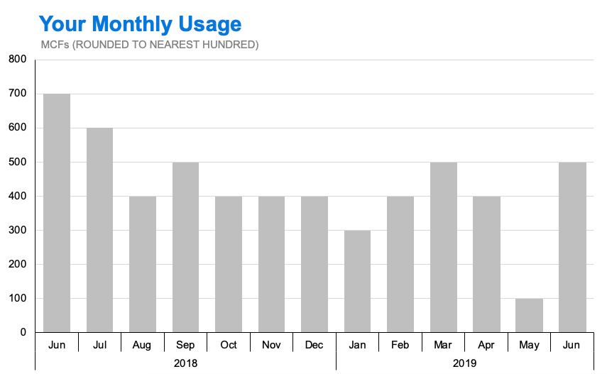
So as to protect the utility company in question, I’ve recreated the chart below, as faithfully as possible. (There are, of course, many changes I would make in order to render this a storytelling with data-esque visualization, but for the purposes of this discussion it’s important that you see the chart as close to its original, “true” form as possible.)

The chart from Mark’s utility bill, recreated from the original photograph as posted on Twitter.

The chart from Mark’s utility bill, recreated from the original photograph as posted on Twitter.

The internet immediately latched onto the seemingly absurd collection of months portrayed in this chart. The bill, dating from June of 2019, included 13 prior months of usage from as early as August of 2016, as recently as March of 2019, and in a random order.

Soon, our non-U.S.-based friends pointed out that the dates made even less sense to them, as (of course) their convention is not to show dates in MM/YY format, but in YY/MM format.

And with this, the truth of the matter became obvious: the dates were in neither MM/YY format nor YY/MM format; they were in MM/DD format, and excluded labeling the year entirely. 


Whenever we run across these kind of so-called “chart fails,” it helps to keep in mind that whoever created the chart wasn’t setting out to be confusing or deceptive. The utility company clearly wanted its customers to be aware of their recent usage, and went so far as to show that usage in a visual format so that it would be more accessible.

The danger, though, is in the assumptions we make when we are the ones creating the chart. Specifically, in this case, there were likely assumptions made about how much information needed to be made explicit versus how much could be assumed.

The energy company likely thought:

The chart says that it’s showing monthly usage; and, since it shows 13 bars, the homeowner will know, or at least assume, that the bars represent the last 13 months in chronological order.

And in general, yes: that is what our first assumptions would be, if there had been no labels whatsoever. 

In this case, the company chose to label the bars with a MM/DD convention, excluding the year—probably to denote what specific day the meter was last read, or on what specific day the last water bill was issued. But we very rarely see dates in MM/DD format when they cut across two different years. We’re trained to see date formats in the style of XX/YY being representative of months and years, not months and days. To interpret the chart correctly, we would have had to ignore and resist our personal experience with this convention.

So on the one hand, logic told us that the chart showed the last 13 months; on the other hand, our experience and the direct labels told us that it was mistakenly showing us 13 random months. What other elements of the chart, or other design choices, could have nudged us towards one of these interpretations over the other?

Perhaps if the chart had been a line chart rather than a bar chart, we would have been nudged into thinking that the data was being shown over a continuous period of time; this could have been enough to make the chart more easily interpreted.

The original chart recreated as a line, rather than a bar.

The original chart recreated as a line, rather than a bar.

Or, if the labels had used abbreviations for the months, rather than numbers, we almost certainly would  have seen the orderly progression of months more clearly.

The original bar chart, but with the months on the horizontal axis labels shown with three-letter abbreviations instead of numbers.

The original bar chart, but with the months on the horizontal axis labels shown with three-letter abbreviations instead of numbers.

Another solution, one which would have almost certainly eliminated all confusion, would have been to include the actual year in the labels, or as super-categories below the existing labels.

With super-categories for the years along the horizontal axis, confusion is likely minimized.

With super-categories for the years along the horizontal axis, confusion is likely minimized.


We could also ask the question: Do we need to be so precise with our X axis labels that the specific day of the month is shown at all? 

It doesn’t seem like it; especially considering that the data on the Y axis has most likely been rounded off, and is presented to the audience at a very general level. 

Look at the level of granularity on the Y axis; although it ranges from 0.1 to 0.7 (in 1000s of units), every bar is shown at an exact increment of 0.1. It’s unlikely that a homeowner’s actual monthly utility usage is always an exact multiple of 100. 

In this case, the labeling of the specific date on the X axis implies a specificity of data that the Y axis does not support. 

Bar chart with more consistency of specificity between the horizontal and vertical axes.

Bar chart with more consistency of specificity between the horizontal and vertical axes.

The bottom line, though, is that the creator of the chart made assumptions about what they needed to show versus what they could exclude; and in making those assumptions, they inadvertently misled their audience in a manner that was very confusing.


It is important to focus your audience’s attention on your data in your visualizations, and to remove extraneous clutter and distracting elements—including redundant information in labels. This case, however, highlights the danger of taking your assumptions too far, and inadvertently adding confusion rather than clarity.

Sometimes we get so familiar with our own work, and our own data, that we lose track of what is, or isn’t, obvious to other people. During your design process, it can be valuable to get input from people who aren’t as close to your work. This helps to identify, and avoid, situations like this one, where familiarity with the data led to design choices that were confusing, rather than clarifying. 

Putting yourself in the mind of your audience, and soliciting feedback from other people who aren’t as close to your subject, will help you to avoid these kinds of misunderstandings in your own work.


Mike Cisneros is a Data Storyteller on the SWD team. He believes that everybody has a story to tell, and he is driven to find ways to help people get their data stories heard. Connect with Mike on LinkedIn or Twitter.


power pairing: color + words

What is one thing you’ll do differently after learning the storytelling with data lessons?

At the end of our workshops, participants are often prompted to reflect on this question. The resulting discussion usually evolves into things that can be easily integrated into the day-to-day work already being done. One piece of advice we frequently give may surprise you—there are two easy actions that don’t require complicated technical skills! First, adopt the habit of stating your takeaway in words. Second, develop the practice of using color sparingly. Today’s post is a quick illustrative example that puts these tips to use. 

At a recent client workshop, we discussed a visual similar to the one below. It is a snapshot of an organization’s current accounts payable (AP) by vendor at a point in time. At a basic level, the graph is fine. It’s cleanly designed with a left-aligned chart title, data labels incorporated into the bars, and no clutter of gridlines or chart border. The bar chart is easy for me to read—I can quickly see that AP is highest for Microsoft and how incrementally larger it is compared to the other vendors because of the consistent baseline (the y-axis). 

 
Picture1.png
 

What I can’t easily see is what I should take away from this chart. At client workshops, we often don’t have this important context—because of this, we often show multiple approaches for highlighting different potential takeaways. Below you’ll see several strategies for employing color and words in this visual. In each of these, notice how the words set up your expectations for what’s emphasized in the graph and color used sparingly indicates where to look in the visual. 

If the audience is interested in the highest spend, I could emphasize the largest vendor:


Perhaps the audience will be more curious where AP is concentrated. I could instead focus attention on the top vendors:


What if the conversation is about expectations—is this spend surprising or unsurprising? I might add additional context with super-categories—useful if the audience is unfamiliar with these vendors’ services—grouping and employing similarity of color and position to visually tie the text to the data it describes. 


Consider pairing color and words in your visuals to be more effective when communicating for explanatory purposes with data. You can practice employing this technique with this community exercise or download the data file to explore the above graphs. Bonus: you don’t need fancy tools to do either of these things!

declutter! (and question default settings)

Decluttering is having a major moment.

Fans of Netflix’s Tidying Up with Marie Kondo have been inspired by guru Kondo’s Japanese-based method of clearing out the clutter in their homes. The benefits are huge. Devotees report living more peacefully and co-existing better with their partners. The key element? Actively working to identify and eliminate anything that doesn’t “spark joy.”

We can apply this same thought process to our data visualizations.

When it comes to clutter in our visuals, we challenge you to regularly examine what specific elements aren’t adding information. What’s making it harder for our audience to get at the data? When we identify and remove clutter from our visuals, the data stands out more.  

We’ve discussed this topic frequently. In this video, Cole provides five tips for how to avoid clutter in visuals; SWD book and workshops each have an entire section focused on decluttering. We don’t intend to create cluttered visuals—rather they often materialize when we don’t take a step back and question our tools’ default settings. Today’s post illustrates one such example and the benefit we can reap from decluttering.

I recently encountered a visualization similar to the following graph. This shows the percentage of babies born within a 24-hour period, broken down by day of the week (having welcomed a baby several months ago, all things maternity still linger in my various news feeds). I recognize this graph: it’s what happens when I put data into Excel and create a stacked bar chart with default settings.

 
Picture2.png
 

This caught my eye not because of the topic but because of how much time it took me to figure out what information it was trying to convey. What should I do with this? There’s a lot competing for my attention in this chart and distracting me from the data.

Spend a moment examining this graph and take note of which specific elements are challenging. Make a list: what might we eliminate or change to reduce cognitive burden?

I came up with eight specific design changes I would make. How does my list compare with yours?

  1. Remove the chart border as it isn’t adding informative value. Often, we use a border to differentiate parts of our slide/visual. In most cases, we can better set them apart with white space.

  2. Delete the gridlines. Will the audience be physically dragging their fingers across the y-axis to identify an exact value? If that level of specificity is important, label the data point(s) directly.

  3. Be sparing in use of data labels. Use them in cases where the exact values are important to the audience. Otherwise, remove and use the axis instead.

  4. Thicken the bars. While there are no hard and fast rules, the bars should be wider than the white space between them so we can more easily compare. In this case, the superfluous white space can be reduced.

  5. Title the axes appropriately. Exceptions are rare for omitting an axis or chart title. Don’t make the audience do work to figure out what they’re looking at, and instead make a habit of titling appropriately to enable the audience’s understanding before they get to the data. Let’s take two related steps here:

    1. Use a more descriptive y-axis title: Instead of the vague %, we can eliminate the guesswork and be more specific: % of total births. While we’re at it, let’s drop the unnecessary trailing zeroes from our y-axis labels.

    2. Clean up x-axis: Diagonally rotated text is slower to read. We can abbreviate the days of the week so they render horizontally. A super-category (such as Weekday or Weekend) could also simplify the process of taking in the information.

  6. Move the legend directly next to the data it describes. This alleviates the work of referring back and forth between the legend and the data.

  7. Use color sparingly. There are so many colors in this graph that our attention is scattered and it’s hard to focus on any one thing. Depending on what we want our audience to take from the graph, we can use color more effectively to focus attention on those pieces only.

  8. Add a takeaway title. Don’t assume that two different people looking at this same graph will walk away with the same conclusion. If there is a conclusion the audience should reach, we should state it in words with an effective takeaway title.

Each step seems relatively minor on its own, but check out the impact when I apply all eight steps simultaneously:


Now we can more easily see that babies delivered on a weekend are more likely to arrive during the early hours of the day (midnight - 6am), compared to weekday deliveries. Related note: this dataset didn’t include the absolute number of babies born each day. Ideally, we’d want that information for context, but for the purposes of this illustrative example, we’ll assume the numbers are large enough to accurately compare across days of the week.

By reducing clutter, the audience can use their precious brainpower to decide what potential actions might be warranted, rather than trying to figure out how to read the graph. Taking time to modify the default settings means we can focus on the data and the message.

In my case, I might have wanted to get some extra rest on the weekends as my due date approached! As it turned out, baby Henry arrived safe and sound among the 17% of Thursday babies born in the 12am-5:59am window.

UPDATE: You can download the file for a further look at how I tackled this in Excel.

For more on the power of decluttering, check out these prior posts:
Declutter this graph: an example of eliminating unnecessary elements
Minor changes, major impact
How to declutter in Excel (with tactical step-by-steps)


Elizabeth Ricks is a Data Visualization Designer on the Storytelling with Data team. She has a passion for helping her audience understand the ’so-what?’ as concisely as possible. Connect with Elizabeth on LinkedIn or Twitter.

March dataviz madness: table vs graph

March madness is here—this three-week period when college basketball fever sweeps the States on the path to crowning the NCAA national champion. We’re pulled into the drama and tension of a single elimination tournament (who will emerge as the Cinderella team to upset a No. 1 seed?) and the stakes are high for teams: one sub-par performance and you’re out.  

When it comes to communicating with data, the stakes can also be high. Maybe not quite as ruthless as a single elimination tournament (one ineffective graph usually doesn’t mean our season is over) but a subpar visual might mean a missed opportunity for our audience to make a data-driven decision.

In data visualization, well-designed visuals are buzzer beating 3-pointers: they capture our attention because they get the main point across quickly and effectively. In today’s post, we’ll look at a dataviz match-up: will it be the table or the graph for communicating an underlying message?

Imagine you’ve encountered the following table: either in a live setting (someone has shown this on a PowerPoint slide) or own your own (said PowerPoint slide has been emailed to you).

 
table.png
 

What’s your initial reaction to this much data? If you’re like me, you’d probably groan and move on, totally disregarding all the hard work that was done behind the scenes to produce this table. Ouch.

When deciding whether to use a table or a graph, consider what the audience needs to do with the data: Do they need a certain level of detail? Are there different units of measure that need to be relayed together? Will they need to refer to a specific line of interest or compare things one by one? If yes, then a table may meet those needs. However, if there’s an overarching message or story in the data, think about making it visual for your audience.

Back to our match-up—imagine that the underlying story is that in recent years, packaging costs have increased at a higher rate and are projected to exceed budget at the end of the fiscal year. Refer back to the tabular data—how long does it take you to find the data that supports this?

Contrast that time-consuming process with the visual below, where I’ve visualized the relevant pieces and added explanatory text and focus through sparing color to make the data more accessible:

 
after visual.png
 

So what is the appropriate use case for a table? When your audience needs detail on specific values or when you have multiple units of measure to report simultaneously. In my previous roles, we used tables frequently in monthly status meetings when the main goal was for participants to give updates on their lines of business and participants wanted to be able to go row by row (or column by column) and refer to specific lines of data. Over time we realized many of these tables weren’t being used and we’d push them to the appendix—they remained there for reference but weren’t competing for attention with the main takeaways.

While we won’t know who wins it all in March Madness until the national championship on April 8, in this match-up we can choose a clear winner: the graph!

In fact, the graph will typically win when there’s an overarching message in the data. A well-designed graph simply gets that information across more quickly than a well-designed table. Don’t make your audience do more work than necessary to understand the data!

For more examples of how to consider if a table is more effective than a graph, check out our previous posts:


Elizabeth Ricks is a Data Visualization Designer on the Storytelling with Data team. She has a passion for helping her audience understand the ’so-what?’ as concisely as possible. Connect with Elizabeth on LinkedIn or Twitter.

three tips for storytelling with qualitative data

Do you find yourself needing to communicating with qualitative data? This post discusses three best practices when communicating with qualitative data—effectively using color, reducing text and considering if audience needs quantitative context—and illustrates through example.

Read More

animating data

When presenting live, you have a ton of opportunity to build a graph or a story piece by piece for your audience. Check out the 90-second video in this post illustrating an example of how we do this at storytelling with data.

Read More